library(tidyverse)
setwd("C:/folder/isee-analysis/")
nh2007 <- load("C:/folder/isee-analysis/nh2007.Rdata")Hands-on Activity 1
Introduction
Goal
At the end of this exercice you should have a project folder created for the analysis. The folder should contains a git repository, th a script/ folder containing the starting script (starting_script.R) and a R/ folder containing descriptive_stats.R with 3 functions.
Tasks
- Setup a reproducible project for the analysis
- Use
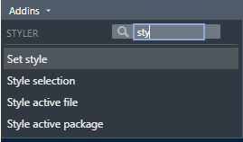
styler::to improve the script - Make your first git commit
- Create two simple functions for descriptive statistics
Starting the project
You should have downloaded the dataset and the script for this workshop if you followed the preworkshop instructions. If you didn’t please go check them and make sure that you already have git installed:
If you wish to recreate the NHANES data by yourself, please have a look at the script in data-raw/nhanes.R in the workshop’s GitHub repository
The first step is to create a folder to gather all the files that we will create for the analysis, you can call it NHANES/ , isee-young-ws8/ or workshop/ it does not matter.
Next we should intialize git within the project folder.
Initialize git repository
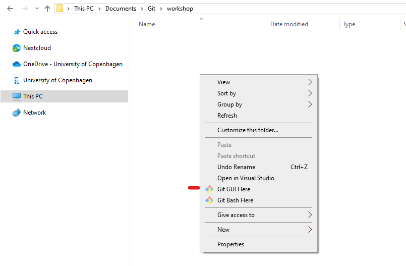
Navigate to the newly created folder, it should be all empty. You can right click in the folder and click on Git GUI here.
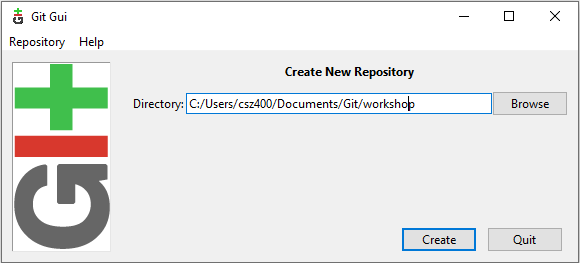
This will open a small widow where we can create a new git repository. The name of the workshop folder should already be there but you can add it manually if needed. You can also launch Git GUI directly from Windows start menu.
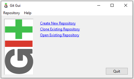
Once the repository is created you should see the main Git GUI interface which look like that:
![]()
The interface is divided in several parts:
- show the files in your working folder
- will display modifications to file that can be staged
- show the files in the staged area and ready to commit
- is where you have tot entre the comit message before commiting the staged files
Please note the “Rescan” button which actualise the state of the working folder in order to see any new modifications done to the files (shortcut: F5).
We can keep this windows open and we will return to it as we advance throught the workshop and need to commit modifcations.
Before adding things to git we need to configure you credentials. Click on Edit > Options to open the following window:
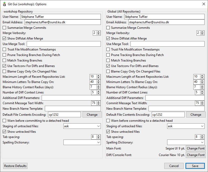
Here you can setup your User Name and Email both for the curent proejct or for all git projects
This step can also be done using by typing the following command in the git command line namely Git Bash.
# GIT bash
git config --global user.name "First Last"
git config --global user.email "first.last@example.com
Tip
You can also initialize a git repository when creating a new R Studio project.
Create a Rstudio project
Now let’s open RStudio to also initiate a Rproject. Click on “New project” in the project menu on the top right corner. Then select “Project in existing directory” and indicate the path of the workshop folder. The project should open itself.
Each RStudio project can be configured. You can either click on the .Rproj file within RStudio or click on “Project option” in the “Tools” menu.
It’s usally better to turn off the saving of the workspace to .Rdata as this prevent old data from previous computations to be loaded automatically each time you open the project which can cause a lot of issues. It’s always better to rerun the scripts form scratch.
Adding folder and files
Now that we have setup both Git and RStudio, let’s organise the project by creating folders and files within the project folder.
- Folders:
data/: the two datasets nh2007 and nh2009 can be put hereR/: keep the folder empty for nowscripts/: copy starting_script.R here
- Files:
README.md: at the root ot the project folder. You can open it in R Studio and add a very short description of the project.scripts/README.md, optional to add some information on the script we can find in this folder
.gitignore: at the root of the project folder. It can contain a list of files that git should ignore. You can open it in RStudio and add the following lines:
# History files
.Rhistory
.Rapp.history

# Session Data files
.RData
.RDataTmp

# User-specific files
.Ruserdata

# RStudio files
.Rproj.user/

# R Environment Variables
.Renviron
This will prevent git from following the modification of these files that are only temporary and not related to the analysis.
The folder should look like that:
Files added by git
Project
├── .git/ <-- Git repository stored here (eg data about changes), hidden folder
├── R/
├── data/
|   ├──  nh2007.Rdata
|   └──   nh2009.Rdata
scripts/
|   ├──starting_script.R
|   └──  README.md
├── .gitignore
├── Project.Rproj
└── README.md
You first commit
It’s time to save in Git the initial state of the project. Switch to the Git GUI windows.
Unfortunately nothing is showing up. It’s because git need to actualise the list of files in the working directory. To do so click on the “Rescan” button. Now all the files and folders should appears in the unstage part of Git Gui. Click on them to show the changes and state of each files.
To commit the file, we have to put them in the staged area by clicking on “Stage to commit” in the “Commit” menu (Shortcut Ctr+T ). Put all the files and folder in the staged area.
Prepare the commit by adding a commit message like: “Initial commit” or “Create project”. Then click on the commit button.
Congratulation all the modifications are now saved 🥳.
If you want to see the saved modification, you can open the repository history by clicking on “View all branch history” in the “Repository” menu.

Improve the script
Loading the data
It’s time to look at the analysis script. You can try to make it run as it is.
The first 3 lines look like that:
Exercice: Can you spot the issue there? How can we improve the loading of the data within the project directory?
Solution
Since we have setup RStudio and we are working within a project and the working directory is the project folder. Therefore we can just specify the path to load the data as a relative pathe (e.g. path within the project):
load("data/nh2007.Rdata")This will work on any computer with the same project sturcture. Relative paths can also used for any files, including to source R scripts.
Script style
Question: What can you notice regarding the coding style used in the script?
- Is it consistent?
- Does it match the tidyverse style guidelines?
# ...
nh2007$id<-factor(nh2007$id)
nh2007$gender<-factor(nh2007$gender)
# ...
nh2007$asthma<- nh2007$asthma%in%1
nh2007$cancer<-nh2007$cancer%in%1
nh2007$cancer <- nh2007$cancer %in% 1
# ....
model.1a <- glm(asthma ~ barium + age_screening + gender,data=nh2007)
model.1.b <- glm(heart_failure ~ barium +age_screening+gender, data = nh2007)
model.1.c<-glm(coronary_heart_disease ~barium + age_screening + gender,data=nh2007)
lead2a <- glm(asthma~lead + age_screening + gender, data = nh2007)
Solution
We can notice:
- Inconsistent spacing in the formulas
- Variations in the names of the models
- General lack of comments
- A lot of copy pasting to repeat the same actions for many variables
First, we can use styler to reformat the whole code:
The code will look much better:
# ...
nh2007$id <- factor(nh2007$id)
nh2007$gender <- factor(nh2007$gender)
# ...
nh2007$asthma <- nh2007$asthma %in% 1
nh2007$heart_failure <- nh2007$heart_failure %in% 1
nh2007$coronary_heart_disease <- nh2007$coronary_heart_disease %in% 1
nh2007$heart_attack <- nh2007$heart_attack %in% 1
nh2007$stroke <- nh2007$stroke %in% 1
nh2007$chronic_bronchitis <- nh2007$chronic_bronchitis %in% 1
nh2007$cancer <- nh2007$cancer %in% 1
# ....
model.1a <- glm(asthma ~ barium + age_screening + gender, data = nh2007)
model.1.b <- glm(heart_failure ~ barium + age_screening + gender, data = nh2007)
model.1.c <- glm(coronary_heart_disease ~ barium + age_screening + gender, data = nh2007)
lead2a <- glm(asthma ~ lead + age_screening + gender, data = nh2007)
We can further change the models names to make them more consitent and informative:
model_barium_asthma <- glm(asthma ~ barium + age_screening + gender, data = nh2007)
model_barium_hf <- glm(heart_failure ~ barium + age_screening + gender, data = nh2007)
model_barium_chd <- glm(coronary_heart_disease ~ barium + age_screening + gender, data = nh2007)
model_lead_asthma <- glm(asthma ~ lead + age_screening + gender, data = nh2007)
This steps is actually optionnal as we will see how to avoid this in the second activity. Now the script should work and is a cleaner. Instead of saving the script as a new file we can save the modifications in git: let’s do a second comit!
First save the script, then switch to Git Gui, click on rescan (or F5). Now starting_script.r should appear as unstaged file and you can see the modification you just made to the file on the right side. If you like the modifications, you can add the modified script to the staged area (see You first commit). Add a commit message like “Apply tidyverse style guide” and commit. In the history you will see that you second commit has been added on top of the first one.
Notice that if you right click on the first commit you have many options like: navigate in your history, change the copy of the files you are working on, revert change, etc. This is outside of the topic of this workshop, but you can read more about it on the following page: https://git-scm.com/book/en/v2/Git-Basics-Undoing-Things
Create a function
Let’s move on the final step of this exercice. As we notice, many steps in this script are repetitives. This is probably fine for this small script, but not so much when you will have 1 000+ lines to modify.
Form lines 41 to 76, the script is doing some simple summary statistics, let’s create functions to simplify theses lines.
Question: Look at the provided R code. What patterns or repetitive tasks do you notice?
Solution
- Frequency tables and bar plots for factors and logical
- Means, standard deviations, quantiles, and histograms for numerical.
Exercise: Write a simple function to compute a frequency table with NA values included.
To find the steps that you need to put in the body of the function, you can first try to do a frequency table on one variable of the dataset. When it’s working, copy paste the steps in the function’s body and replace the variable names wiht variable. Before testing the function, you need to run the lines with the function definition to load the function in R memory.
compute_table <- function(variable) {
  # Steps to do on variable
}
Solution
# Define the function
compute_table <- function(variable) {
  # Return frequency table as a dataframe
  table(variable, useNA = "always")
}

# Call the function with gender variable
compute_table(variable = nh2007$gender)Exercise: Create a similar function for numeric variables. The function need to return the mean, standard deviation, and quantiles.
Solution
compute_numeric <- function(variable) {
  # Compute the statistics
  mean_value <- mean(variable, na.rm = TRUE)
  sd_value <- sd(variable, na.rm = TRUE)
  quantiles <- quantile(variable, na.rm = TRUE)

  # Return statistics, in a list
  list(
    "mean" = mean_value,
    "sd" = sd_value,
    "quantiles" = quantiles
  )
}
In this case, we need to return multiple results. To do so, all the results need to be regrouped in a list or a dataframe because functions can only return one object.
Exercise: Join together the two functions in one function that can handle both categorical and numerical variables.
To test variable type you can use the following code:
is.numeric(variable)
is.factor(variable)
is.logical(variable)
Solution
compute_descriptive_stats <- function(variable) {
  # Function to call if the variable is numeric
  if (is.numeric(variable)) {
    statistics <- compute_numeric(variable)
  }

  # Function to call if the variable is a factor or a logical
  if (is.factor(variable) || is.logical(variable)) {
    statistics <- compute_table(variable)
  }

  statistics
}

# Test the function
compute_descriptive_stats(nh2007$age_screening)
compute_descriptive_stats(nh2007$gender)
Now we can rewrite the previous lines like that:
compute_descriptive_stats(nh2007$gender)
compute_descriptive_stats(nh2007$education)
compute_descriptive_stats(nh2007$education_child)
compute_descriptive_stats(nh2007$asthma)
compute_descriptive_stats(nh2007$heart_failure)
compute_descriptive_stats(nh2007$coronary_heart_disease)
compute_descriptive_stats(nh2007$creatinine)
compute_descriptive_stats(nh2007$lead)
compute_descriptive_stats(nh2007$barium)
compute_descriptive_stats(nh2007$cadmium)
Extensions of the functions
Discuss which possible extensions and modifications are possible:
- create plots for each type of variable using ggplot2
- adding other statistical measures
Exercise: create a new function that create plots for each type of variable using ggplot2.
Solution
# Descriptive univariate graphs
compute_descriptive_graph <- function(variable) {
  # Histogram
  if (is.numeric(variable)) {
    p <- ggplot2::ggplot(mapping = aes(x = variable)) +
      ggplot2::geom_histogram()
  }

  # Barplot
  if (is.factor(variable) || is.logical(variable)) {
    p <- ggplot2::ggplot(mapping = aes(x = variable)) +
      ggplot2::geom_bar()
  }

  p
}

# Test the function
compute_descriptive_graph(nh2007$creatinine)
compute_descriptive_graph(nh2007$lead)
compute_descriptive_graph(nh2007$barium)
compute_descriptive_graph(nh2007$cadmium)
The little p is needed at the of the function to return the graph. If you remove it you will see that nothing will be return. This is because a function return the last output from it’s body.
Optionnal exercise: create a new descriptive statistics function that includes at least one additional calculation not covered previously.
Before break
Move all the new functions to a file in the R folder “descriptive_stats.R”.
Add a line to source “R/descriptive_stats.R” in “starting_script.R”:
source("R/descriptive_stats.R")Save the change in git and commit the newly created functions.